Pretraining and fine-tuning

Learn from unlabeled histories by reconstructing hidden values, then adapt the model to a labeled outcome.

The event-history model combines account context with an ordered transaction sequence to predict disputes and merchant repeats for every transaction at a shared snapshot cutoff. The account example adds outcomes at different levels. Both need settled labels. Your application may have years of payment histories but far fewer completed outcome windows.

Give those histories a learning role by hiding selected amounts or merchants and recovering them from the remaining context. Then use labeled payments to adapt the learned context to the operational outcome.

Pretraining learns from relationships in a broad collection of records. Fine-tuning starts from those learned weights and adapts the model to a specific task. In relflow, both use model.fit(...); the data and reconstruction objectives determine what the model learns.

Stage	Data	Objectives
Self-supervised pretraining	Records without task labels	Reconstruct sampled observed values with rf.Mask(rate=..., reconstruct=True).
Supervised fine-tuning	Labeled task records	Predict always-hidden transaction labels with mask=True, optionally retaining reconstruction objectives.
Resume a run	The same training task	Restore the model, optimizer, scheduler, and loop progress from a full Lightning checkpoint.

Figure 1: The same transaction fields under each stage. Pretraining reconstructs sampled amounts and merchants; fine-tuning makes them visible and hides every dispute label; prediction omits the labels.

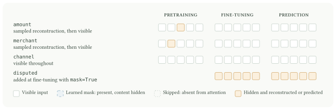
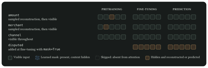
Pretraining is optional. A supervised model can also start from newly initialized weights. An ordinary float mask, such as mask=0.15, only supplies input dropout; pretraining needs reconstruct=True to create an objective.

Reconstruction recovers amounts and merchants already present in the saved sequence. The supervised labels keep their definitions from Profile context and a second outcome: one cutoff per observation and a 30-day window after it.

Once the model has learned from your histories, you can adapt it with labeled examples or keep it fixed and test exported embeddings as inputs to separate task predictors. Evaluate both choices against the existing task workflow on the same held-out observations. The event-history guide explains how to define observations, decision cutoffs, and future outcome windows.

Pretrain on histories

Keep the account profile and full transaction sequence from the event-history example. Omit the two future outcomes for this stage. Observed amounts and merchants provide their own supervision when selected values are hidden:

account_age_days: 420
trxns:
  - booked_at: "2026-03-28T09:00:00"
    amount: 24.00
    merchant: Harbor Internet
    channel: direct_debit
  - booked_at: "2026-04-28T09:00:00"
    amount: 24.00
    merchant: Harbor Internet
    channel: direct_debit
  - booked_at: "2026-05-27T08:00:00"
    amount: 32.00
    merchant: Station Cafe
    channel: card
  - booked_at: "2026-05-28T09:00:00"
    amount: 24.00
    merchant: Harbor Internet
    channel: direct_debit

import relflow as rf

model = rf.Model.xs(
    account_age_days=rf.Number,
    trxns=rf.Branch(
        length=32,
        overflow="tail",
        booked_at=rf.DateParts(
            dateparts=["day_of_month", "day_of_week", "hour_of_day"],
        ),
        amount=rf.Number(mask=rf.Mask(rate=0.15, reconstruct=True)),
        merchant=rf.Category(
            mask=rf.Mask(rate=0.15, reconstruct=True),
        ),
        channel=rf.Enum(values=("card", "direct_debit", "bank_transfer")),
    ),
)
pretraining_data = rf.ArrowDataModule(
    train="payments/pretraining/train.parquet",
    validate="payments/pretraining/validation.parquet",
)
model.fit(
    pretraining_data,
    batch_size=128,
    max_epochs=50,
    checkpoint_dir="checkpoints/payment-pretraining",
)
model.save("artifacts/payment-pretrained.rf")

The two paths identify independent, application-supplied Parquet files with this richer record structure. Histories are sorted oldest to newest for overflow="tail". The profile, booking calendar, and channels remain visible while selected transaction amounts and merchants are hidden. Keep preparation consistent through the preprocessing pipeline.

Each sampled value is predicted from the remaining context; unselected values remain inputs. These fractional reconstruction policies also sample during validation and test, but are inactive during ordinary prediction. See Masking and reconstruction for selection and stage rules.

Fitting restores the best validation checkpoint before the artifact is saved. See Training options for checkpoint selection.

Adapt to a labeled task

For this adaptation, add a settled Boolean disputed label to every transaction. Each answers the common-cutoff question above. All labeled transaction positions contribute to the supervised objective.

Pretraining and fine-tuning splits must respect the same evaluation boundaries; pretraining on held-out accounts or future observations changes what the downstream evaluation measures.

Load the pretrained artifact, remove its sampled reconstruction policies, and add a supervised label:

finetuned = rf.Model.load("artifacts/payment-pretrained.rf")
reconstructed_inputs = rf.where("address").is_in(
    [
        rf.Address("trxns", "amount"),
        rf.Address("trxns", "merchant"),
    ]
)
finetuned.update(reconstructed_inputs, mask=False)
finetuned.extend(
    rf.where("address") == rf.Address("trxns"),
    disputed=rf.Boolean(mask=True),
)

Amount and merchant remain visible inputs. mask=True keeps every dispute label out of the input and uses it as supervision. If the target already exists, update its mask to True instead of adding it again.

The profile, booking dates, and channel fields stay in place. To adapt to the merchant-repeat outcome instead, add repeats_next_30_days=rf.Boolean(mask=True) to trxns and supply every transaction’s label for the same future window. The event-history guide shows both supervised outcomes together.

Figure 2: The same transaction sequence supplies reconstruction context and each transaction’s dispute prediction.

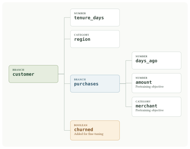
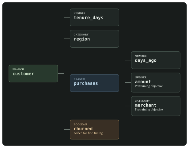
Schema edits rebuild modules and retain state entries whose names, types, and tensor shapes still match. The new target starts with newly initialized state; changing widths, field types, or structure can also reinitialize incompatible parts. Keep existing addresses and geometry stable when reusing a pretrained model. Adding a field can change context and reduction behavior even when existing weights transfer. Schema mutation describes these boundaries.

Start a new training run

Start a new fit with labeled Parquet files supplied by your application. The call binds a fresh optimizer to the edited model, including its new target. A smaller learning rate is a starting point to evaluate:

finetuning_data = rf.ArrowDataModule(
    train="payments/finetuning/train.parquet",
    validate="payments/finetuning/validation.parquet",
)
finetuned.fit(
    finetuning_data,
    batch_size=128,
    learning_rate=1e-4,
    weight_decay=0.01,
    max_epochs=20,
    checkpoint_dir="checkpoints/payment-finetuning",
)
finetuned.save("artifacts/payment-disputes.rf")

This starts new optimization from the transferred model state. Use ckpt_path with a full Lightning checkpoint when resuming the same task, including its optimizer and loop progress. Reapply processors and desired compilation after loading and schema edits. Pass any scheduler to this fit call; it is not inherited from pretraining. For DDP, every rank must construct the same final schema.

Fine-tuning here updates the model end to end, including the new decoder and existing encoders. Loaded vocabularies and Number normalization statistics also continue learning from training observations; loading does not freeze them. Validation, test, and prediction reuse that state. For a fixed feature extractor, continue with embeddings: add embed=True to this saved model’s root or trxns branch, export in prediction mode, and fit a separate predictor without updating the exporting model. This lets you test the learned context for another outcome before choosing to fine-tune it.

At inference, omit disputed from every transaction and keep the transaction records. The schema address is /trxns/disputed; output format 2 returns each retained transaction’s result inside predictions.trxns, with inferred: true at every position. See Prediction output.

Keep auxiliary objectives deliberately

To retain amount reconstruction alongside dispute, keep that policy when adapting the pretrained artifact. Replace the earlier finetuned.update(reconstructed_inputs, mask=False) call with:

finetuned.update(
    rf.where("address") == rf.Address("trxns", "merchant"),
    mask=False,
)
finetuned.update(
    rf.where("address") == rf.Address("trxns", "amount"),
    weight=0.1,
)

Then add the dispute target and start the new run as above. Keeping the amount policy preserves its trained decoder; removing reconstruction and later reenabling it creates a new decoder. Both amount and dispute losses are now optimized. weight scales the amount loss rather than its sampling rate or a fixed fraction of the combined loss.

Compare fine-tuning against the same supervised task trained from scratch. Use the same held-out data and dispute metric: pretraining loss and fine-tuning loss have different objective sets and are not directly comparable. Retaining auxiliary objectives may help or hurt the task, so evaluate that choice rather than assuming pretraining guarantees a better model. See Evaluation.

Evaluate vocabulary coverage

For large-vocabulary reconstruction, report how many selected answers the model can express as well as how well it predicts them. For example, monitor .trxns.merchant/validate.coverage.content alongside .trxns.merchant/validate.nll.content and .trxns.merchant/validate.accuracy.all. The Category metrics and Cluster metrics define these denominators and count unavailable targets explicitly.

An unknown Category or Cluster target contributes no label gradient. Forcing its prediction to be uniform over known labels would teach a different task, not recover the missing answer. With no known targets, conditional reconstruction quality is NaN; zero coverage means the validation objective is unmeasurable, not that the model reconstructed everything perfectly. Cluster balancing and adaptive-cluster updates also exclude unknown answers. Do not select a checkpoint from such a conditional score without checking coverage.

Vocabulary growth can change the evaluated known-target population between epochs. NLL can increase when newly admitted, difficult labels join it even if predictions on the old labels improve. The summed validation loss is not a coverage-adjusted model-quality score. Keep a fixed validation source, monitor coverage, and compare known-target quality at comparable coverage. If necessary, retain a fixed cohort of training-established labels for an additional stable diagnostic; do not populate the model vocabulary from validation or test data.

Random reconstruction masks introduce another source of variation. For a repeatable diagnostic, supply application-owned Boolean selection fields and use Mask(query=..., reconstruct=True). This fixes selected coordinates; it does not freeze vocabulary growth or make unknown answers learnable. Keep any held-out calibration set separate from model selection, and evaluate downstream confidence separately for familiar and unseen input identities.

P062 isolates vocabulary coverage with fixed query-selected masks and checks that rebatching the same targets cannot change the reported counts or conditional scores. P065 tests Cluster coverage.

P066 separately checks cold Category inputs across successive training cohorts. It currently exposes a remaining failure: admitting an input identity can change reconstruction NLL without an optimizer step, even at complete target coverage. Target coverage does not measure input familiarity. Keep input cohorts separate when assessing pretraining stability; fixed masks alone cannot remove this source of drift. Initialization alternatives that pass the admission check have failed other learning proofs and are not enabled in the model.

Set metrics count positive memberships rather than scalar targets. A partial-OOV Set retains its known positive and negative supervision; dropping the whole set would discard valid evidence. An all-OOV set still supplies known negatives when annotations are complete. Report member coverage, complete-set coverage, exact-set accuracy, and micro F1 together. Empty sets are valued, complete annotations, although an all-empty evaluation has no positive-member denominator. These semantics are not appropriate for incompletely annotated labels without further masking.

Next, reuse the learned context as input to separate predictors, with the exporting model kept fixed.