Model tree

How a schema describes one observation: fields, branches, names, addresses, size, and context settings.

The schema describes one observation. For account review, it identifies the transaction sequence available at a cutoff and the later outcome for each record. Fields describe values; a branch groups related values; the model root combines them to predict a target.

Follow one observation

Take the model from Add transaction history, which reads the three-transaction record shown there:

import relflow as rf

model = rf.Model.xs(
    trxns=rf.Branch(
        length=32,
        overflow="tail",
        booked_at=rf.DateParts(
            dateparts=["day_of_month", "day_of_week", "hour_of_day"],
        ),
        amount=rf.Number,
        merchant=rf.Category,
        disputed=rf.Boolean(mask=True),
    ),
)

Figure 1: Each node has an address formed from the names along its path. The root is anonymous.

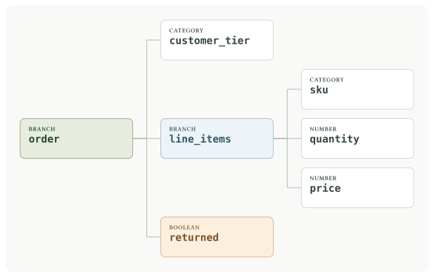
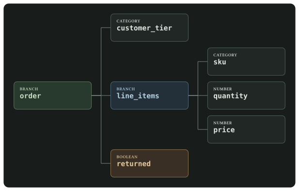
The timestamp, amount, and merchant at one list position belong to the same transaction. The latest payment appears once at the end of trxns; the root contains no second amount or merchant. mask=True hides and supervises every transaction’s dispute value, and prediction can omit disputed from every record.

This structure lets the model learn both which fields occur together in an event and how behavior varies across the history. With the default reduction, the branch passes a learned context summary to the root; that summary is trained for the prediction objectives. A calculated spending total or purchase count remains a separate feature the application can supply.

Account attributes such as tenure or plan belong at the level that owns that context. If supplied for a payment decision, use their values as known then; an account’s plan can change. Keep event-specific values with the transaction they describe.

length=32 limits the history to 32 transactions. With oldest-to-newest input, overflow="tail" keeps the latest ones. Sorting and excluding future records belong in application data preparation, as Prepare observations describes. Omitting length retains all history items and lets each batch determine its width; see automatic lengths and limits.

Names and addresses

The parent names each child: amount=rf.Number creates an amount field. Use the bare class for defaults; call it for options, as in disputed=rf.Boolean(mask=True) in the transaction branch.

An address identifies a location in the schema. Use one argument per child name; RelFlow adds the leading slash and separators:

root = rf.Address()                                      # /
trxn_amount = rf.Address("trxns", "amount")
selected = model.select(rf.where("address") == trxn_amount)

The second address is /trxns/amount. The target is /trxns/disputed. Addresses identify schema locations in configuration, metrics, and mutations, even when a query reads another source path. rf.Address is a string subclass and serializes as a plain string in schema configuration. Prediction output uses ordinary child names in its result tree and path segments in representation records.

The root is anonymous, has address /, and represents one observation. The diagram label payment is illustrative, not a model option or address prefix. A field named name is an ordinary child, with address /name. Repeated data belongs in a child branch. A child branch reads a list even when length=1.

Definitions take no positional arguments or name option. Use fields for generated schemas or a child name that collides with configuration:

transactions = rf.Branch(
    length=32,
    fields={"amount": rf.Number, "description": rf.Category},
)

Reusing a definition creates independent named nodes and learned modules; it does not share weights. See Prepare observations for how names and nesting select source values.

Choose a size

rf.Model.xs(...), .sm(...), .md(...), .lg(...), and .xl(...) supply architecture defaults. Start with xs or sm to establish a working model, then compare larger sizes on validation data. Schema size, vocabularies, and decoded fields also affect memory and compute.

The presets leave collection lengths, overflow, queries, masking, datatype options, optimizer settings, and runtime settings to the application. See Model presets for the size table, node-local overrides, and checkpoint rules. For schemas stored in YAML, see Model templates.

Configure the context

Use rf.Model(...) with required d_model, n_layers, and n_heads to choose the architecture directly. d_model is the shared embedding width. Root encoder settings apply to the root; child branches have their own settings.

Setting	Controls
attention	Branch encoder: "mha", "gqa", "mqa", or None.
n_layers, n_heads, dropout	That branch’s encoder.
ffnx	Feed-forward hidden width as a multiplier of d_model; default 8 on every node.
reduction	Context passed to the parent; default rf.Attention().
length	None by default: retain all records; a positive integer sets a hard limit.
overflow	Only with a finite limit: keep first records ("head", the bounded default), last records ("tail"), or raise ("error").
mask	Inputs to hide or reconstruct; see Masking and reconstruction.
embed=True	Export a representation; see Reusable representations.

Set a positive integer ffnx on a root, branch, or tensorfield to change that node’s feed-forward width. Each child keeps its own default unless configured. A branch uses it for its sequence encoder, coordinate encoder, and learned reduction. A tensorfield uses it for its query decoder and aligned context projection:

model = rf.Model(
    d_model=64,
    n_layers=2,
    n_heads=4,
    ffnx=8,
    trxns=rf.Branch(
        length=32,
        overflow="tail",
        ffnx=4,
        booked_at=rf.DateParts(
            dateparts=["day_of_month", "day_of_week", "hour_of_day"],
        ),
        amount=rf.Number,
        merchant=rf.Category,
        disputed=rf.Boolean(mask=True, ffnx=6),
    ),
)

RelFlow’s hidden neural activations use tanh GELU and its neural normalization uses RMSNorm with epsilon 1e-5. Pretrained text encoders retain their own architectures.

Encoder and reduction settings are separate. attention=None disables encoder attention while leaving the reduction in place. rf.Mean() averages present inputs and adds a learned count lane; reduction=None preserves routed child slots. Attention reductions have their own settings and inherit omitted heads/dropout from the branch. See Branch for the full contract.

Padding and structurally skipped inputs do not contribute to attention or mean pooling. An explicit null remains a modeled value state; see Value state. A decoder pools representations along its ancestor path and can condition learned queries on visible siblings at matching coordinates. Tree connections show ownership; database joins belong in preprocessing.

Only declared options are accepted. Use description for notes. A leaf’s active=False retains it in the schema while excluding it from execution. Change an existing model through mutation methods.

To follow the evidence through this tree, continue with How fields interact, Branch summaries, and Tree routing and decoding.