Averaging supplied squared deviations

Isolate population-variance decoding after each item’s squared deviation has already been calculated.

Seed 3500 on gpu: 1 of 1 behavioral checks met. See the measurements below. The experiment code has changed since this run; these measurements describe its earlier version.

Insights

Providing squared deviations tests averaging; it does not show that the model can calculate variance from raw values. The generator has already centered and squared each value. The model receives those sufficient statistics and learns to decode their average as population variance.

That makes the case a useful diagnostic beside raw-value variance: if this succeeds while the raw route fails, investigate centering or the learned nonlinear interaction before blaming final reduction. Mean averages encoded tokens, so numerical decoding still has to work. The accuracy gate does not independently establish permutation behavior, varying collection lengths, or handling of missing values, and it supplies no evidence that the model learned the preprocessing operation.

Setup

"""Supplied squared deviations isolate collection averaging.

Mean learns population variance once squared deviations are supplied.

Run: uv run python proofs/run.py P009"""

from __future__ import annotations

from collections.abc import Iterator

import lightning.pytorch as lit
import numpy as np
import torch
from reporting import report

import relflow as rf

PROOF_ID = "P009"
ITEMS = 8

Examples

Targets use mask=True; the labels below are supervision hidden from the encoder.

Unit squared deviations

items:
  - {squared_deviation: 1.0}
  - {squared_deviation: 1.0}
  - {squared_deviation: 1.0}
  - {squared_deviation: 1.0}
  - {squared_deviation: 1.0}
  - {squared_deviation: 1.0}
  - {squared_deviation: 1.0}
  - {squared_deviation: 1.0}
variance: 1.0

Eight supplied squared deviations of 1.0 have a population average of 1.0.

A smaller supplied spread

items:
  - {squared_deviation: 0.04}
  - {squared_deviation: 0.04}
  - {squared_deviation: 0.04}
  - {squared_deviation: 0.04}
  - {squared_deviation: 0.04}
  - {squared_deviation: 0.04}
  - {squared_deviation: 0.04}
  - {squared_deviation: 0.04}
variance: 0.04

The numerical decoder must distinguish this average of 0.04 from the first record.

Unequal deviations with the same average

items:
  - {squared_deviation: 0.25}
  - {squared_deviation: 1.75}
  - {squared_deviation: 0.25}
  - {squared_deviation: 1.75}
  - {squared_deviation: 0.25}
  - {squared_deviation: 1.75}
  - {squared_deviation: 0.25}
  - {squared_deviation: 1.75}
variance: 1.0

The per-item contributions differ, but they still average to 1.0. Every record already supplies the centering and squaring operation; these examples illustrate that diagnostic boundary.

Synthetic data and controls

def dispersion_records(*, rows: int, seed: int) -> Iterator[dict]:
    """Draw rows whose location and spread are statistically independent."""
    rng = np.random.default_rng(seed)
    for _ in range(rows):
        basis = rng.normal(size=ITEMS)
        basis -= basis.mean()
        basis /= np.sqrt(np.mean(np.square(basis)))
        location = float(rng.uniform(-0.8, 0.8))
        scale = float(rng.uniform(0.12, 1.25))
        values = location + scale * basis
        items = [{"squared_deviation": float(np.square(value - location))} for value in values]
        yield {"items": items, "variance": scale * scale}


def prediction(model: rf.Model, observations: list[dict]) -> np.ndarray:
    inputs = [{"items": row["items"]} for row in observations]
    output = model.predict(inputs)["predictions"].to_pylist()
    return np.asarray([row["record/variance"]["content"] for row in output], dtype=np.float64)


def rmse(actual: np.ndarray, predicted: np.ndarray | float) -> float:
    return float(np.sqrt(np.mean(np.square(actual - predicted))))


def score(*, train: list[dict], test: list[dict], predicted: np.ndarray) -> dict[str, float]:
    """Compare held-out RMSE with the constant training-target mean."""
    actual = np.asarray([row["variance"] for row in test], dtype=np.float64)
    baseline = rmse(actual, float(np.asarray([row["variance"] for row in train], dtype=np.float64).mean()))
    measured = rmse(actual, predicted)
    return {"rmse": measured, "baseline_rmse": baseline, "nrmse": measured / baseline}

Model tree

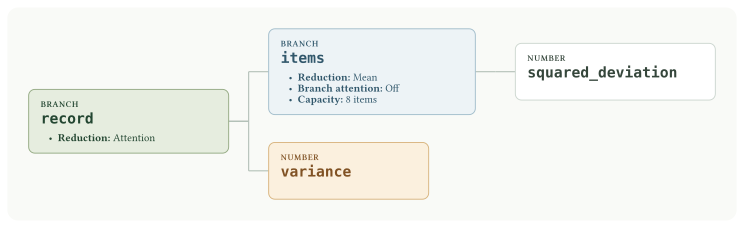
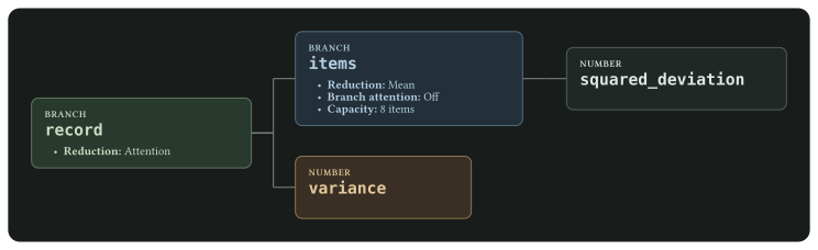
Figure 1: Mean averages eight encoded squared deviations with item attention disabled; root Attention feeds the variance decoder.

How it works

The generator computes (value - mean(value)) ** 2 before encoding. The item branch uses attention=None and rf.Mean(); the root uses learned attention to predict the average of eight supplied squared deviations.

Mean averages encoded tokens, so the decoder still has to learn their numerical interpretation. Passing this diagnostic supports reduction and decoding of sufficient statistics. It does not prove learned centering or squaring; the raw-value variance proof checks those requirements.

Training and evaluation

def run(seed: int, steps: int | None, accelerator: str) -> tuple[dict, dict]:
    lit.seed_everything(seed, workers=True)
    # Split seeds are independent; rerunning a generator reproduces the same records.
    train = list(dispersion_records(rows=768, seed=seed + 1))
    test = list(dispersion_records(rows=384, seed=seed + 3))
    model = rf.Model(
        d_model=32,
        n_layers=2,
        n_heads=4,
        reduction=rf.Attention(n_layers=2),
        batch_size=64,
        optimizer=lambda module: torch.optim.Adam(module.parameters(), lr=0.001),
        items=rf.Branch(length=ITEMS, n_layers=2, attention=None, reduction=rf.Mean(), squared_deviation=rf.Number),
        variance=rf.Number(mask=True, objective="mse"),
    )
    datamodule = rf.SyntheticDataModule(
        model=model,
        train=lambda: dispersion_records(rows=768, seed=seed + 1),
        validate=lambda: dispersion_records(rows=192, seed=seed + 2),
        seed=seed,
    )
    trainer = lit.Trainer(
        accelerator=accelerator,
        devices=1,
        max_epochs=-1,
        max_steps=350 if steps is None else min(steps, 350),
        logger=False,
        enable_progress_bar=False,
        enable_model_summary=False,
        enable_checkpointing=False,
        deterministic=True,
        num_sanity_val_steps=0,
    )
    trainer.fit(model, datamodule=datamodule)

    # Evaluate held-out answers and retain their original labels in corruption controls.
    measured = score(train=train, test=test, predicted=prediction(model, test))
    metrics = {"measured": measured, "steps": trainer.global_step}
    checks = {"Variance nRMSE below 0.20": bool(measured["nrmse"] < 0.2)}
    return metrics, checks

Evidence

Latest full run

Seed 3500, gpu, recorded 2026-09-15T02:19:57.574262+00:00. Outcome: met.

Source fingerprint: 9794c74e27d86088dfb4ea8d03abccb0a8bc826edc859bf652613b0ffc95017b. Python 3.12.6; Torch 2.12.0.

Measurement	Value
measured	rmse: 0.0101722; baseline_rmse: 0.480072; nrmse: 0.0211889
steps	350

Behavioral checks

Behavioral check	Outcome
Variance nRMSE below 0.20	Met

Recorded results.

Remaining work

Repeat this control across seeds and broaden collection lengths and edge cases. Keep population-versus-sample variance semantics explicit, and retain the raw-value comparison when claiming that dispersion was learned from inputs.

The family’s promotion target is at least three core seeds and ten lightweight calibration seeds.

Reproduce

Run by stable ID from the repository root:

uv run python proofs/run.py P009

Or run the self-contained script directly:

PYTHONPATH=proofs uv run python proofs/aggregation/supplied_squared_deviations.py

Add --accelerator gpu for CUDA or --seed 42 for another seeded experiment. --steps 2 checks execution with a short training budget; it is recorded as a smoke run.

Download the complete proof.

if __name__ == "__main__":
    report(PROOF_ID, run, seed=3500)